Show the code
pacman::p_load(ggstatsplot,tidyverse,gganimate,performance, ggdist,highcharter,patchwork)The task is to reveal the patterns of resale prices of public housing property in 2022 by residential towns and estates in Singapore. The intention is to help the users to have better data discovery experience by using relevant interactive visualisation techniques.
The raw data is downloaded from Resale flat princes based on registration date from Jan-2017 onwards from Department of Statistics, Singapore. The data is cleaned up to focus on resale prices of 3/4/5 Room in 2022 before importing.
Install and load all the relevant libraries to use for visualization.
pacman::p_load(ggstatsplot,tidyverse,gganimate,performance, ggdist,highcharter,patchwork)Raw data is imported from resaleFlatPrices2022.csv and put into resaleFlatRaw data frame.
resaleFlatRaw <- read_csv("data/resaleFlatPrices2022.csv",show_col_types = FALSE) After the raw data is imported, all the number variables are converted into integers type so the statistical analysis can be applied to them. Data conversion of years to months is also done for remaining_lease variable. The resale_price_sqm variable is created to do better comparison between different flat types.
First the remaining_lease column is extracted into remaining_lease_year and remaining_lease_month and converted into integer variables. Next, the NA is replaced with 0 for remaining_lease_month. Lastly, remaining_lease_months variable is created by adding up remaining_lease_year and remaining_lease_month into months.
resaleFlat <- resaleFlatRaw %>%
  mutate(resale_price=as.integer(resale_price)) %>%
  mutate(floor_area_sqm=as.integer(floor_area_sqm)) %>%
  mutate(resale_price_psm = resale_price/floor_area_sqm) %>%
  extract(remaining_lease,c("remaining_lease_year","remaining_lease_month"),
          "([0-9]{2}) years ?([0-9]{2})?",convert=TRUE) %>%
  mutate(remaining_lease_month=replace_na(remaining_lease_month,0)) %>%
mutate(remaining_lease_months=(remaining_lease_year*12)+remaining_lease_month) %>% select(-c(remaining_lease_year,remaining_lease_month))The 1st visualisation is to display the mean resale price per sqm for individual town so that the user can determine the mean resale price fluctuation across towns. The final visualisation is sorted in ascending order for mean resale price per sqm.
options(highcharter.theme = hc_theme_smpl(tooltip = list(valueDecimals = 2)))

resaleFlatmean <- resaleFlat %>% group_by(town) %>%
  summarise(mean_resale_price_psm = mean(resale_price_psm))

resaleFlatmeanSorted = resaleFlatmean[order(resaleFlatmean$mean_resale_price_psm),]

hc <- resaleFlatmeanSorted %>%
  hchart('column', hcaes(x = town, y = mean_resale_price_psm)) %>%
  hc_title(text="HDB Mean Resale Price Per Sqm in 2022", align = "center")

hc
Based on the bar chart above, it can be observed that central area has highest mean resale price per sqm while woodlands area ha s lowest mean resale price per sqm. It can deduced from the chart that most of the central region planning areas have higher mean resale price per sqm compared to other regions.
The 2nd visualisation is to investigate whether mean resale price per sqm in 2022 is increased from mean resale price per sqm in 2021 which is $4,839 according to the MND. So, this is the test.value that will be used.
p1 <- gghistostats(data = resaleFlat, x = resale_price_psm,
                   xlab = "Resale Price Per Sqm",
                   title = "Distribution of Resale Price Per Sqm for HDB in 2022",
                   test.value = 4839,
                   centrality.parameter = "mean")
p1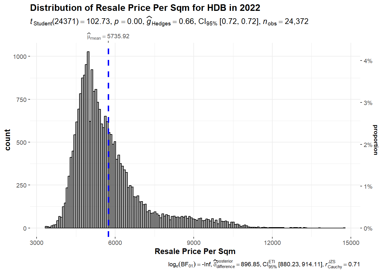
As you can see from the graph above, the mean value of resale price per sqm in 2022 is significantly higher than the mean value of resale price per sqm in 2021. There is also extreme evidence provided by Bayes factor that the mean resale price per sqm in 2022 is higher compared to 2021.
The 3rd visualisation is compare the mean resale price per square meter for different flat types. It is also to check that the differences in mean resale price per sqm between flat types is statistically significant or not.
ggbetweenstats(
  data = resaleFlat,
  x = flat_type,
  y = resale_price_psm,
  type = "p",
  mean.ci = TRUE,
  xlab = "Flat Type",
  ylab = "Resale Price Per Sqm",
  title = "Comparison of Resale Price per Sqm across Flat Types in 2022"
)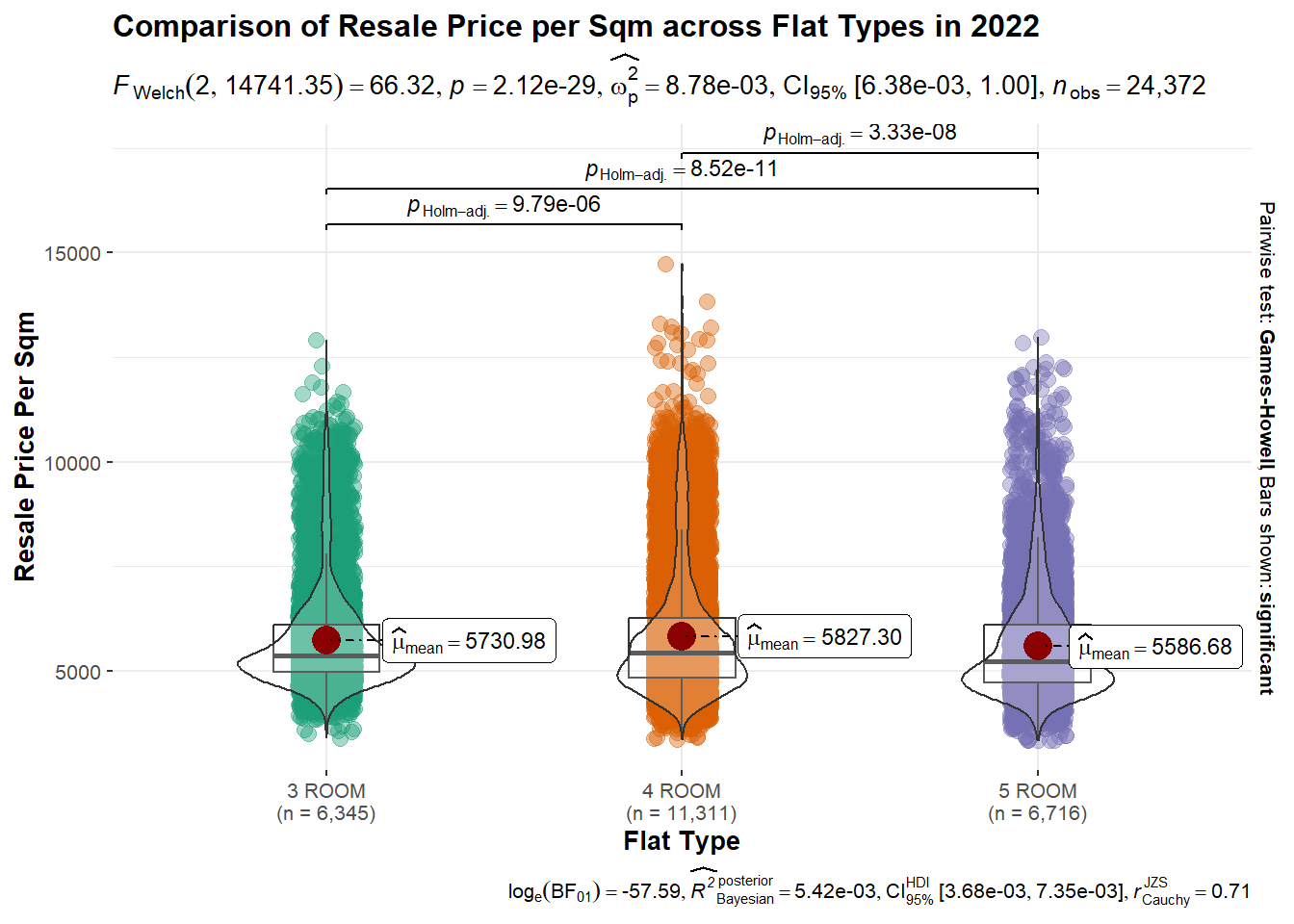
From the above chart, the mean resale price per sqm across flat types across different flat types is comparable to one another. Moreover, the distribution pattern across different flat type is similar.
The 4th visualisation is to reveal the relationship between resale price per square meter and floor area in square meter.To do the visualisation, resale price per sqm and floor are in sqm are binned 4 bins.
resaleFlat1 <- resaleFlat %>%
  mutate(resale_price_psm_bins = cut(resale_price_psm, breaks = c(0,3333,6183,9033,11883,14733))) %>%
  mutate(floor_area_sqm_bins = cut(floor_area_sqm, breaks = c(0,30,60,90,120,160)))

ggbarstats(resaleFlat1,
           x = resale_price_psm_bins,
           y = floor_area_sqm_bins,
           xlab = "Resale Price per Sqm",
           ylab = "Floor Area Sqm",
           legend.title = "Resale Price per Sqm Bins",
           title = "Resale Price per Sqm vs Floor Area Sqm")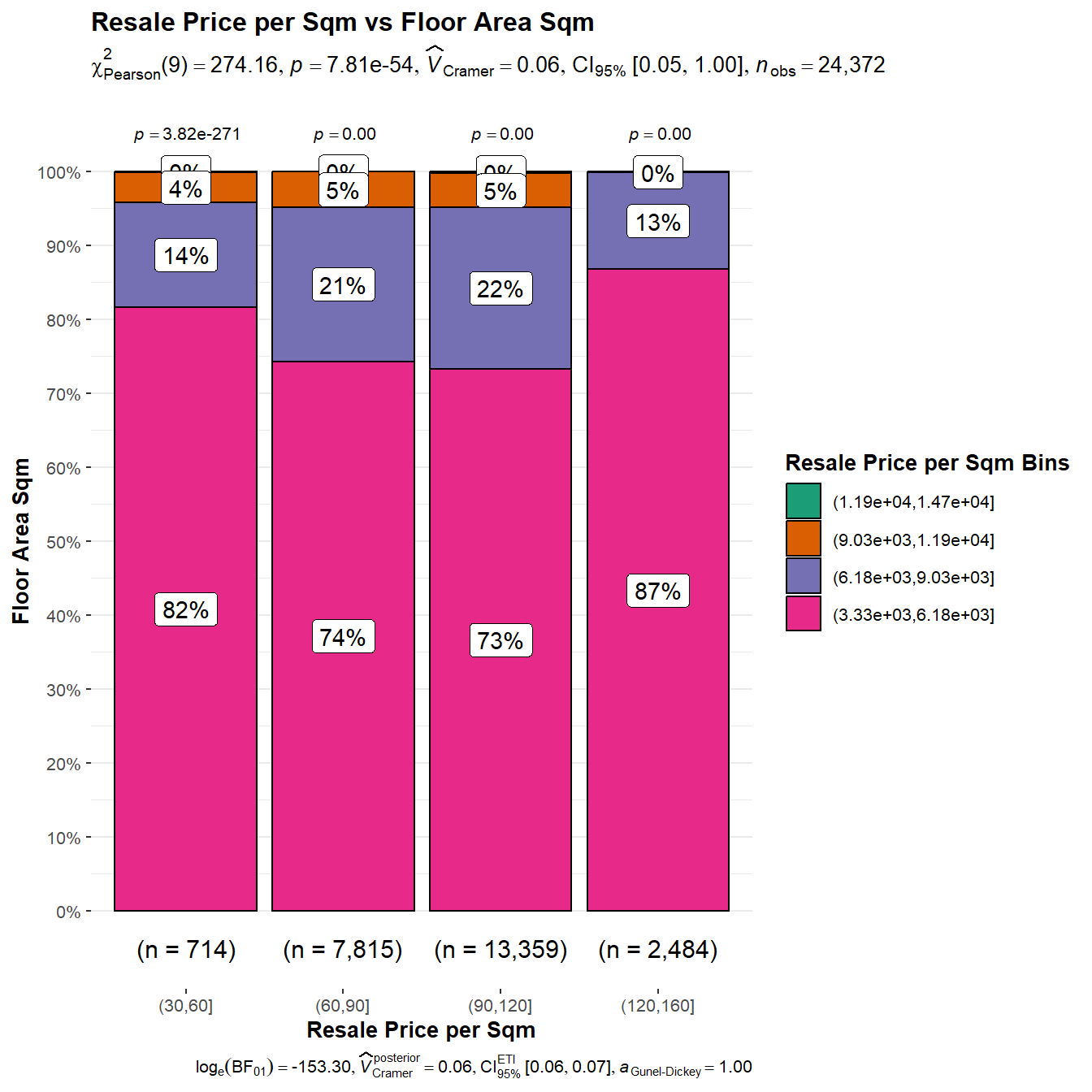
From the resulting chart, it can be seen that most of the 30-60 sqm and 120-160 sqm of floor area are sold at lower resale price per sqm compared to 60-120 sqm of floor area. The highest resale price per sqm for 120-160 sqm of floor area is between $6183 and $9033 while The highest resale price per sqm for other floor area is between $9033 and $11883 It can be deduced that resale price per sqm for smaller room can be higher than the bigger room.
Multiple Linear Regression Model
The multiple linear regression model is applied for resale price with different parameters such as flat model, storey range and so on.
model <- lm(resale_price_psm ~ month + town + storey_range +
              floor_area_sqm + flat_model + remaining_lease_months, data = resaleFlat)
model
Call:
lm(formula = resale_price_psm ~ month + town + storey_range +
    floor_area_sqm + flat_model + remaining_lease_months, data = resaleFlat)

Coefficients:
                     (Intercept)                      month2022-02
                        1718.924                            40.341
                    month2022-03                      month2022-04
                          72.452                           148.689
                    month2022-05                      month2022-06
                         181.689                           251.271
                    month2022-07                      month2022-08
                         295.773                           306.500
                    month2022-09                      month2022-10
                         386.920                           438.789
                    month2022-11                      month2022-12
                         453.446                           490.672
                       townBEDOK                        townBISHAN
                        -280.283                           784.252
                 townBUKIT BATOK                   townBUKIT MERAH
                        -864.458                          1003.111
               townBUKIT PANJANG                   townBUKIT TIMAH
                       -1435.395                          1538.595
                townCENTRAL AREA                 townCHOA CHU KANG
                        1394.661                         -1665.866
                    townCLEMENTI                       townGEYLANG
                         240.825                           355.438
                     townHOUGANG                   townJURONG EAST
                        -827.032                          -921.221
                 townJURONG WEST               townKALLANG/WHAMPOA
                       -1330.377                           681.763
               townMARINE PARADE                     townPASIR RIS
                        1318.809                          -962.931
                     townPUNGGOL                    townQUEENSTOWN
                       -1445.643                          1093.563
                   townSEMBAWANG                      townSENGKANG
                       -1594.610                         -1521.392
                   townSERANGOON                      townTAMPINES
                          29.056                          -504.296
                   townTOA PAYOH                     townWOODLANDS
                         493.312                         -1543.226
                      townYISHUN              storey_range04 TO 06
                       -1189.617                           185.602
            storey_range07 TO 09              storey_range10 TO 12
                         339.910                           419.979
            storey_range13 TO 15              storey_range16 TO 18
                         523.890                           739.191
            storey_range19 TO 21              storey_range22 TO 24
                        1025.045                          1164.541
            storey_range25 TO 27              storey_range28 TO 30
                        1384.468                          1761.702
            storey_range31 TO 33              storey_range34 TO 36
                        1885.688                          2026.521
            storey_range37 TO 39              storey_range40 TO 42
                        2207.980                          2450.416
            storey_range43 TO 45              storey_range46 TO 48
                        2662.916                          3437.031
            storey_range49 TO 51                    floor_area_sqm
                        2908.513                            -6.039
         flat_modelAdjoined flat                    flat_modelDBSS
                         174.458                          1322.658
              flat_modelImproved     flat_modelImproved-Maisonette
                          52.275                          1647.555
               flat_modelModel A      flat_modelModel A-Maisonette
                          33.494                          1145.945
              flat_modelModel A2          flat_modelNew Generation
                          78.316                           232.176
     flat_modelPremium Apartment  flat_modelPremium Apartment Loft
                         258.855                           981.651
            flat_modelSimplified                flat_modelStandard
                         395.000                           157.229
               flat_modelTerrace                 flat_modelType S1
                        4035.515                          2062.109
               flat_modelType S2            remaining_lease_months
                        1950.796                             5.038
Next step is to check the multicollinearity of different parameters to resale price.
check_c <- check_collinearity(model)
check_c
# Check for Multicollinearity
Low Correlation
Term VIF VIF 95% CI Increased SE Tolerance
month 1.03 [1.02, 1.05] 1.02 0.97
floor_area_sqm 1.46 [1.44, 1.48] 1.21 0.69
remaining_lease_months 2.47 [2.42, 2.52] 1.57 0.41
flat_model 8.75 [8.55, 8.96] 2.96 0.11
Tolerance 95% CI
[0.95, 0.98]
[0.67, 0.70]
[0.40, 0.41]
[0.11, 0.12]
Moderate Correlation
Term VIF VIF 95% CI Increased SE Tolerance Tolerance 95% CI
storey_range 1.93 [1.90, 1.97] 1.39 0.52 [0.51, 0.53]
town 6.81 [6.65, 6.97] 2.61 0.15 [0.14, 0.15]plot(check_c)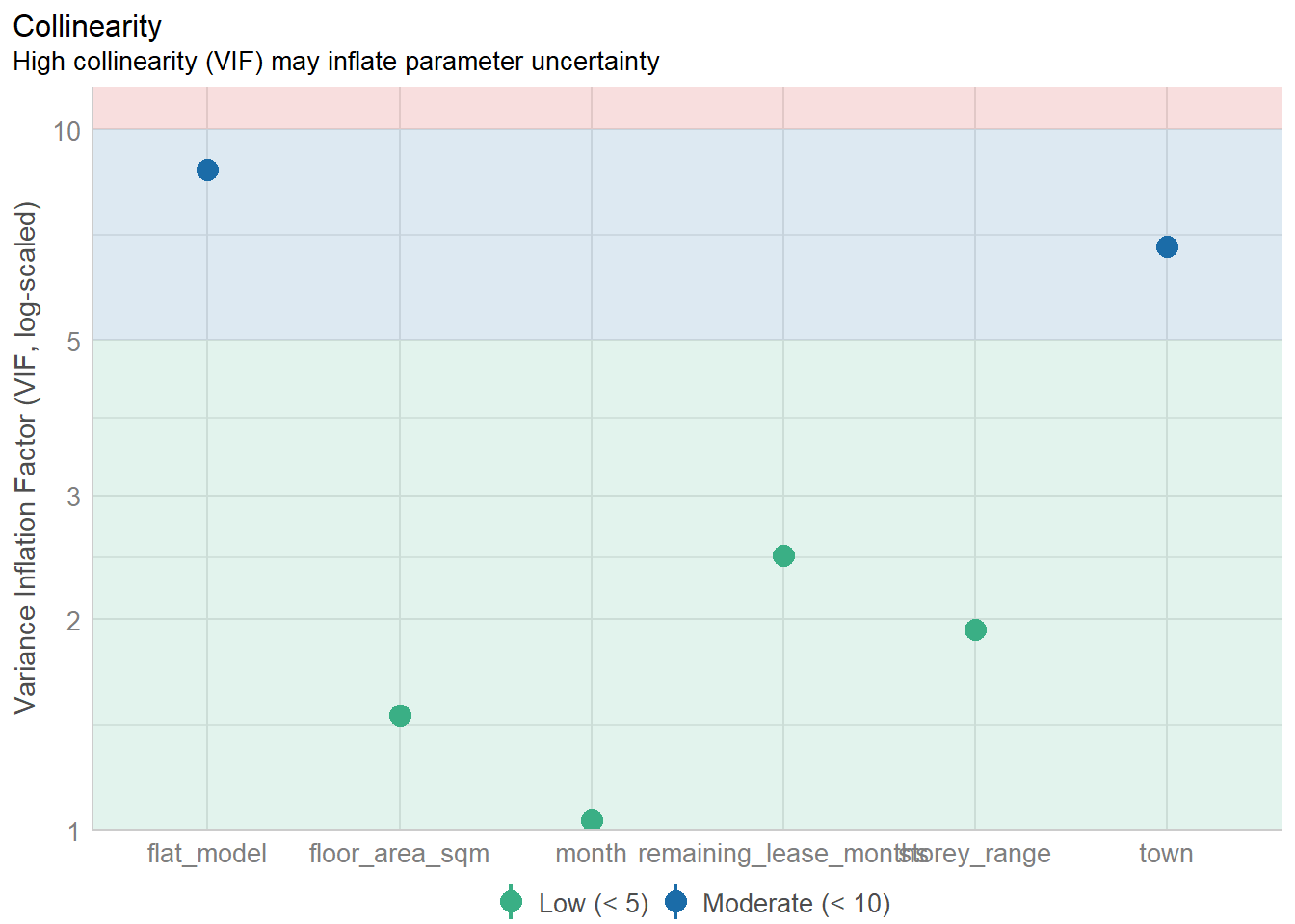
From the plot, it is illustrated that flat model and town plays more significant role to resale price per square meter while the rest of the parameters has less significant role.
Next is checking normality of residuals for the model.
check_n <- check_normality(model)
plot(check_n)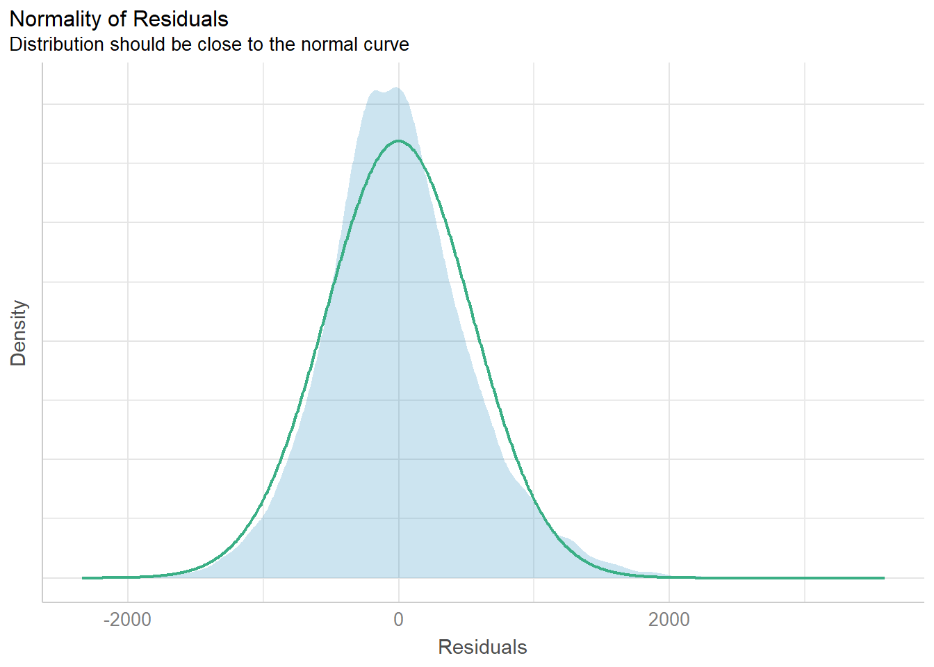
From the plot it can be said that the the model residual failed to conform to normality assumption because residual histogram (in cyan colour) is not closed to the theretical histogram (i.e in green).
Visualizing the Uncertainty of Point Estimates
This visualisation is to display the distribution of resale price per sqm by flat model.
resaleFlat %>% ggplot(aes(x = flat_model,
             y = resale_price_psm)) +
  stat_gradientinterval(
    fill = "skyblue",
    show.legend = TRUE
  ) +
  labs(
    title = "Visualising confidence intervals of resale price per sqm of HDB in 2022",
    subtitle = "Gradient + interval plot") +
    xlab("Flat Model") + ylab( "Resale Price per Sqm") +
  theme(plot.title = element_text(size=16, hjust=0.5),
        axis.title.x = element_text(size=15),
        axis.text.x = element_text(angle=45, hjust=1),
axis.title.y = element_text(size=15)) 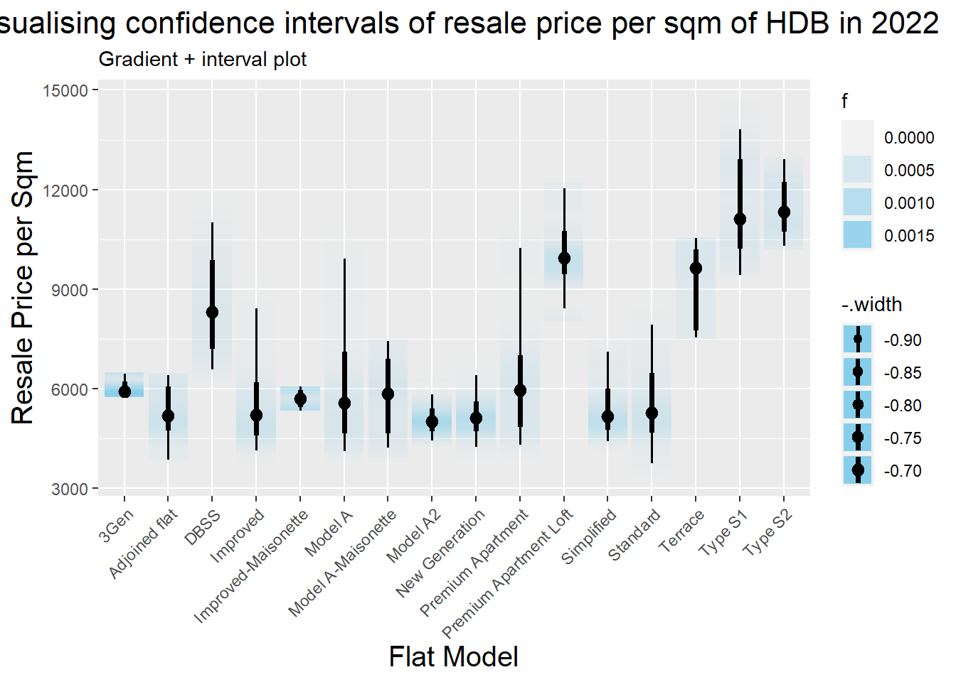
The confidence interval for different flat type is more or less similar to each other. Type S1 and S2 has higher resale price per sqm compared to the rest.
Take-home exercise 3 can help me to familiarize with different analytics approach for statistical testing, building the linear regression model and visualising uncertainty. It also introduce me different libraries and functions for visualisation and statistical analysis.